IOT BASIC

CONTENTS
1 What is an IOT?. . . . . . . . . . . . . . . . . . . . . . . . . . . . . . . . . . . 2
2 Where is the EEV IOT used? . . . . . . . . . . . . . . . . . . . . . . . . . . . . . 2
3 Historical Background and Alternative Amplifiers for UHF TV . . . . . . . . . . . . . . . 2
3.1 FromVHF toUHF . . . . . . . . . . . . . . . . . . . . . . . . . . . . . . 2
3.2 The Klystron . . . . . . . . . . . . . . . . . . . . . . . . . . . . . . . . . 2
3.3 Solid-State . . . . . . . . . . . . . . . . . . . . . . . . . . . . . . . . . 4
3.4 The Tetrode . . . . . . . . . . . . . . . . . . . . . . . . . . . . . . . . . 4
3.5 The IOT . . . . . . . . . . . . . . . . . . . . . . . . . . . . . . . . . . . 5
3.6 The Diacrode . . . . . . . . . . . . . . . . . . . . . . . . . . . . . . . . 5
4 Detailed Description of EEV IOT Operation . . . . . . . . . . . . . . . . . . . . . . . 5
4.1 Magnet Frame . . . . . . . . . . . . . . . . . . . . . . . . . . . . . . . . 5
4.2 TheEEVIOT . . . . . . . . . . . . . . . . . . . . . . . . . . . . . . . . . 5
4.3 Input Cavity . . . . . . . . . . . . . . . . . . . . . . . . . . . . . . . . . 9
4.4 Output System . . . . . . . . . . . . . . . . . . . . . . . . . . . . . . . 12
4.5 Linearity . . . . . . . . . . . . . . . . . . . . . . . . . . . . . . . . . . 17
5 How to Tune EEV IOT Systems . . . . . . . . . . . . . . . . . . . . . . . . . . . 17
6 Conclusion. . . . . . . . . . . . . . . . . . . . . . . . . . . . . . . . . . . . 19


1 What is an IOT?
The Inductive Output Tube or IOT is a high vacuum,electron tube which works in combination with a
specially designed circuit assembly to provide theheart of a high power UHF amplifier. The tube and
cavity combination, or system (see Fig. 1) is designed to give an 8 MHz pass-band when tuned to any
channel in the frequency range 470 to 860 MHz. The system contains the high negative voltages inside a
safe grounded enclosure. X-ray and RF leakage are reduced to a safe level.
The IOT system must be connected to cooling water and air, the cathode high voltage supply, isolated heater, ion gauge and grid bias supplies at high voltage, and a focus current supply. A peak RF drive
power of up to 1000 W is fed into the input cavity, and up to 100 kW peak UHF power can be taken from
the output coupler to a suitable load or aerial. An interlock protection and control logic system is required to check the availability of necessary services and switch on the amplifier in the correct sequence. In case the tube should flash over internally, a crowbar circuit is required to protect the internal tube structure from follow through currents until the high voltage supply can be disconnected by a normal fast circuit breaker.
2 Where is the EEV IOT used?
The main use for the EEV IOT is in high powered UHF television transmitters, particularly in the USA. There
may also be future uses for the tube in industrial heating, and RF power supplies for physics research
machines. In the 1990s, the IOT almost completely replaced the klystron as the preferred electron tube for the final high power amplifier of UHF television transmitters. It is more efficient than the klystron and reduces energy consumption by 50% for the same transmitter power rating. In addition it is linear enough to permit the combined amplification of sound and vision, which allows medium powered transmitters to be simplified
to the minimum tube complement of one only compared with klystrons, where two are required for separate vision and sound amplification.The IOT is also the best choice for final high power amplification of digital signals in

3 Historical Background and Alternative Amplifiers for UHF TV
3.1 From VHF to UHF
Television transmission began with relatively few channels, and these could be accommodated in VHF
bands I and III between 50 and 260 MHz. The necessary transmitters could be made using coaxial
triodes or tetrodes in coaxial cylindrical line cavities, and the 25 kW maximum vision power could often be
provided by one final stage tube. These transmitters were the first to be replaced by solid-state equipment
in the 1980s and 1990s.
In the 1960s the demand for television services increased, and at the same time there was a requirement for higher definition and colour transmission. It now became necessary to use the UHF bands IV and V to accommodate all the wider channels required by public and commercial broadcasting.
The four main amplifier types (klystron, transistor, tetrode and IOT), shown for comparison in Table 1,
were all invented before this requirement came up, but the klystron amplifier was the obvious choice at
the time. Transistors were very new and only modestly developed; tetrodes could not reliably be made with close spacing until the advent of the carbon grid in the early 1970s. The IOT had not even been considered because of its high drive requirement and the lack of the technology for making a reliable grid.
3.2 The Klystron
The amplifier klystron has large internal spacings and a very high gain, and could be driven by 5 or 10 W
amplifiers using available high frequency miniature gridded vacuum tubes. The poor efficiency of the klystron was accepted because there was no alternative. The klystron also provided poor linearity and it was necessary to amplify the sound and vision separately in two klystrons and combine afterwards to avoid interference (crosstalk or intermodulation product distortion). However, the klystron was very reliable and long-lived.

	Klystron	Klystron sync. Pulsed	Klystron MSDC	Transistor	Tetrode	IOT	Diacrode
Invention	1939	1975	1982	1948	1936	1938	1990
Adoption	1960	1980	1985	1970	1975	1990	1994
Gain (dB)	40	40	40	7	13	20	13
Electrical efficiency (grey and sync.) (%)	9	14	28	16	24	32	29
IPD (dB)	740	740	740	740	750	750	750
Common amplification	no	no	no	yes	yes	yes	yes
Maximum power per device (kW)	70	70	70	0.1	50	110	100
Typical average life (hours)	50 000	25 000	50 000	450 000	15 000	30 000	15 000

Table 1 UHF TV amplifier types

Once the klystron had been adopted for UHF TV transmission, klystron makers and users then worked to improve the performance of their product, particularly in electrical efficiency, to reduce the high running costs and to respond to competition from alternative systems as they came along. At first the klystron was run with a fixed beam power sufficient to provide the sync. pulse power. At this maximum power the basic efficiency of the klystron (35% say) was obtained, but at the mid-grey average signal level the efficiency was only 7%. Basic efficiency was improved to 45% (bringing mid-grey to 9%) by designing for lower gain as higher power drive

amplifiers became available. Then a major step-up in efficiency was achieved by pulsing the beam current  up for the sync. pulse and down to a level sufficient for black for the rest of the picture period; this moved mid-grey level picture efficiencies up to 14%. Finally the multistage depressed collector was added to the klystron with the necessarily greater tube and power supply complexity involved, but a further improvement in efficiency up to 28% for mid-grey level.

3.3 Solid-State

Transistors were soon in use in amplifiers to drive klystrons, and equipment makers were keen to use them in complete transmitters despite their poor efficiency because of their perceived reliability. However, there are fundamental physical limitations to the maximum output powers of individual transistors at UHF. The features that increase output power, i.e. increased junction area and reduced device thickness, also increase capacitance and limit maximum frequency. Further, the skin effect limits the useful junction area to a few microns’ width next to the edge, and the length of edge has to be increased by dividing the junction area into a finger like pattern. The most advanced UHF transistors can now produce of the order of 100 W effective output and are arranged in series/parallel arrays to make modules with 250 W, 500 W, 1000 W outputs. Each device is connected through protective circuitry so that the failure of one device cannot produce an avalanche of destruction through its neighbours. The linearity of such amplifiers is modest, but with multiple modules there is no difficulty providing

separate amplification of vision and sound. The electrical efficiency remains poor, and the capital cost continues high. However, solid-state transmitters are being purchased wherever extreme reliability is thought to be required and only the ‘graceful’ decline in power of multiple device amplifiers can be tolerated.

3.4 The Tetrode

Tetrode electron tubes with thoriated tungsten mesh filaments and molybdenum grids were used for 500 W UHF TV transposers from the late 1960s. In the early 1970s the pyrolytic graphite grid became available and was used in UHF tetrodes with 0.2 mm electrode spacings and peak sync. power outputs of 10, 20 and 30 kW. These devices have to have very high power densities because there are fundamental limitations on maximum internal dimensions. There are risks of parasitic standing waves, or modes, if any internal dimension, such as length or diameter exceeds 1/16 of a wavelength (a rough rule-of-thumb). Also, the finite screen grid end-cap to anode capacitance prevents the current node/voltage anti-node of the tuned circuit being centred on the active area of the tube. Nevertheless, the tetrode is still electrically efficient and linear, and can be used for transmitters up to 30 kW peak sync. vision only or 20 kW peak sync. combined sound and vision amplification. At first smaller tetrodes were used as sound and/or vision driver tubes, but lately solid-state amplifiers have taken over these jobs. The UHF tetrode has never been able to demonstrate lives comparable with the klystron (or IOT), especially above about 15 kW of peak sync. power.

3.5 The IOT

The arrival of pyrolytic graphite on the electron tube scene provided a suitable material for the fine spherical grid closely spaced in front of a spherical indirectly heated dispenser cathode for the IOT. 

The first practical tube to be made was the so-called ‘Klystrode’, a klystron/tetrode hybrid. At that time UHF drive amplifiers were still relatively expensive, and this encouraged the klystrode designers to incorporate regenerative feedback to increase the tube gain; this gave them some inherent hazards of linearity and stability to overcome. The klystrode also encountered serious problems with spurious emission from its grid.

EEV (now E2V Technologies) came next with its IOT, which eliminated the grid emission problem and settled for lower gain, thus avoiding the instability of input cavities using feedback. E2V Technologies had different problems to overcome: the RF drive had to be fed through isolating chokes (or blocking capacitors) to the gun at high negative voltage (735 kV); at first these chokes could not stand high operating temperatures and broke down; the problem was subsequently solved by the use of ceramic chokes. The EEV IOT has provided long life and reliable

operation and has become the preferred tube for most high power UHF TV transmitters.

3.6 The Diacrode

In what is probably the final stretching of the tetrode technology, the Diacrode joins two tetrodes back to back on their common cylindrical axis with a coaxial socket/header on either side of a common anode. The screen grid is connected to both sides, but the control grid and cathode are connected to one side only for cathode heating and cathode drive. With an anode cavity on each side, the tube has achieved the advantage of bringing the current node/voltage antinode to the middle of the screen grid/anode structure.

The diacrode is being applied to a range of combined vision and sound amplification UHF TV transmitters. Its service life will probably be limited to an absolute maximum of about 20 000 hours (about half that of an EEV IOT) by the inevitable depletion of the carburising of the slender thoriated tungsten wire in the mesh cathode.

4 Detailed Description of EEV IOT Operation
In Fig. 2 an IOT system is shown exploded into its major sub-systems:
Magnet Frame;
IOT;
Input Cavity;
Output Circuit consisting of a primary and secondary output cavity.
4.1 Magnet Frame
The magnet frame supports the tube through its lower pole piece. It is shown in Fig. 3, together with the tube pole pieces and drift tubes. The magnetic flux produced by the coils follows the high permeability materials. Between the pole pieces and inside the drift tubes there is a magnetic field to focus the electron beam and prevent it hitting the drift tubes.
The magnet frame supports the secondary output cavity and brings the output coupler to a specified plan position and height.
The frame also provides a system ground connection, and supports customers’ wiring harnesses and other
interfaces.
4.2 The EEV IOT
The EEV IOT is a sealed, high vacuum device, which allows an electron beam to travel from one end to the
other in a precisely controlled way. It is shown separately in Fig. 4.
The electrons are emitted from the spherical front surface of a dispenser cathode (tungsten matrix impregnated with barium aluminate), which is heated from behind by a radiant tungsten heater. The flow of
electrons is controlled by a fine spherical pyrolytic carbon grid spaced close to the cathode. The grid and
cathode are mounted on metal supports which are separated by a hermetic ceramic insulator which is
part of the tube envelope and through which the drive signal passes. The cathode is maintained at735 000 V
by a 3 A DC power supply; the grid is biased at 7100 V with respect to the cathode by an isolated
supply floating on the negative high voltage. This gun is isolated from the grounded IOT body by a hermetic
ceramic insulator covered with convoluted silicone rubber to increase the surface tracking length and
prevent voltage breakdown.

If the grid voltage is made less negative with respect to cathode potential, then more current flows from the cathode. The electric field makes the beam converge into the anode nose where the increasing space charge turns it parallel to the tube axis. The magnetic field shown in the previous section then holds it parallel through the output gap. After the beam has passed the lower pole-piece, where the magnet focus field is removed, it diverges under space-charge repulsion and is dissipated on the inside of the water cooled collector. The current picked up by the body other than the collector can be measured separately by the circuit shown in Fig. 4.

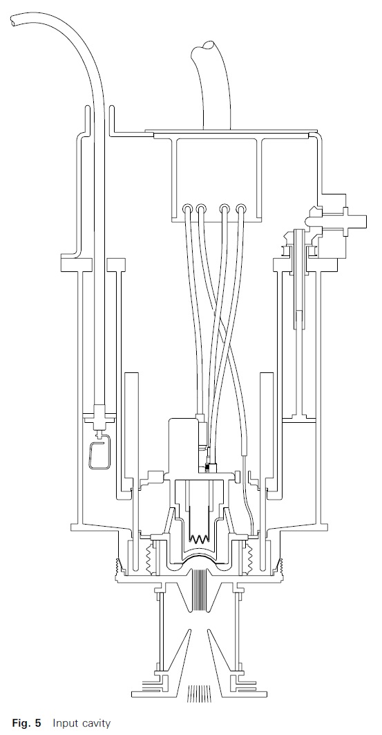
4.3 Input Cavity

The input cavity and the top half of the IOT are shown together in Fig. 5.

4.3.1 Input Cavity Tuning

The input cavity is a medium-Q resonant coaxial line cavity whose volume can be adjusted to tune from

470 to 860 MHz using a 3/4 l mode at the low frequency end and 5/4 l mode at the high frequency end, see tuning curves Fig. 6. The outer case and the adjustable volume of the cavity are at ground potential. The input power is fed in through a grounded coaxial cable to a loop antenna on the cavity side of the movable annular tuning short circuit or door. The input signal causes a current to flow in and out of the end  Capacitance of the loop antenna.

An alternating magnetic field is generated perpendicular to the loop, and this induces a current to flow up the inside cavity cylinder across the underside of the tuning door and down the outside cavity cylinder and vice versa. This excites a resonant standing wave to build up in the cavity over 10 or 20 cycles to a final level in proportion to the input signal. 

The coaxial line continues inside the IOT between the cylindrical supports of the cathode and grid. Because

the gun is at 735 kV, this smaller coaxial line section must be connected to the larger tunable grounded

outer section by a disc shaped section incorporating DC isolating RF chokes, one in the inner line to the

cathode and a second similar one in the outer line to the grid.

The standing wave in the cavity is distorted as it goes through this zig-zag path through the disc shaped region containing the chokes. To explain the tuning procedure, a simplified schematic layout is shown in Fig. 7, in which a straight cavity section with no chokes ends immediately at the grid to cathode gap.

The best input tune is obtained by adjusting the door position for maximum beam current. This occurs when the grid-cathode gap is part way between a voltage node and antinode at a point where the voltage to current ratio exactly matches the impedance of the grid to cathode capacitance.

The lowest frequencies can be tuned using a 3/4l mode with the door movement near mid-range. As the frequency increases the door is tuned to the limit of its range (lowest volume) for 3/4l. Above this frequency the 3/4l current antinode is nearer the gridcathode gap than the door can reach. The door must  now be retracted towards maximum cavity volume position to include an extra half wavelength for the 5/4 l mode. Moving the door from maximum volume to minimum volume now covers the top part of the frequency band on the 5/4 l mode.The cavity design also contains features to overcome two potential problems. The insulating chokes provide a path through which RF energy can escape from the grid-anode cavity into the cathode-grid cavity. At certain frequencies this feedback can be in the correct phase and have sufficient power to cause oscillation of the IOT; the grid-anode cavity has therefore been loaded with ferrite material to absorb sufficient RF energy to make the system stable at all frequencies. Secondly, the input cavity has other resonances than the 3/4 l and 5/4 l modes shown in Fig. 6. However, the design is such that these are not excited if the tuning door is pre-set to the correct position for the drive frequency that is to be used. 

4.3.2 Input Cavity/Junction Box

The input cavity contains inside its grounded lid an insulating junction box for the high voltage supplies.

These supplies arrive along insulated cables inside a grounded flexible conduit which terminates at the lid.

The supplies consist of the high negative voltage, high current supply to the cathode (which also serves

as the heater return), the heater supply, the ion pump supply, and the grid bias. The last three are isolated

supplies floating at high voltage. The grid bias lead passes through a coaxial feed-through capacitor at

the cathode plane to bypass any RF that would otherwise flow back to the supply.

In building up a system, the IOT is equipped with leads, and these are plugged into the junction box once the input cavity has been installed.

4.3.3 Input Cavity/Beam Pulsing

Before the IOT beam can be powered the system must be prepared as described below and as shown in

Fig. 1. The IOT is positioned in the magnet frame; theprimary output cavity is clamped round the tube and

the secondary cavity screwed to the primary; the output coupler at the top of the secondary is joined to a suitable RF load. It is imperative not to draw any electron beam current without the output cavities being in place because only they can contain safely the RF and X-ray radiation (see data sheet). The magnet frame earth and collector lead are connected.

The input cavity is lowered over the tube, the leads connected to the junction box, and the top lid closed

to activate the microswitch safety interlock. The arc detector leads are connected to the monitoring/control circuits.

Water cooling to the collector and body, air cooling to the input and output cavities, and magnetising

current to the frame are switched on.

With all the necessary support services in action, the interlocks will now permit the heater power to be

switched on. After five minutes warm-up, monitoring circuitry will check the readiness of the crowbar to

fire. Then a suitable grid bias (of the order of 7100 V) can be applied and the high voltage switched on. An

idle current of about 600 mA is required as the best amplifier linearity will be obtained in class AB

operation. 

The input cavity is tuned to the chosen channel by adjusting the cavity for maximum beam current on a

low level signal of the appropriate frequency. The two output cavities are now both tuned to the same

frequency and their intercoupling adjusted to give the necessary 6 or 8 MHz pass band at the correct

position with respect to the carrier frequency. The output coupling is also adjusted to give the best flat

response - see section 5.0 for details.

If drive power is now fed to the input cavity at this chosen channel then an alternating UHF voltage is

added to the grid bias to give the total grid voltage with respect to cathode as shown in Fig. 8.

A sync. level signal is shown which takes the grid voltage just up to cathode voltage, beyond which electron current would begin to be collected by the grid. The tube should in general not be driven harder than this to avoid grid heating and consequent grid emission. An intermediate grey level signal is also shown in this diagram.

It can be seen that the beam current increases approximately sinusoidally in the positive going half cycle and is largely suppressed in the negative going half cycle. The electrons released through the grid are accelerated through 35 kV before entering the anode drift tube, and at this energy form bunches denser in the middle and about 100 mm long at mid-range frequencies. It is these bunches that will give up their energy to the output cavity at the output gap.

4.4 Output System

4.4.1 Double Tuned Output

The output system comprising primary and secondary output cavities and the output coupler is shown together with the IOT output section in Fig. 9. A single output cavity across the IOT output gap does not have sufficient bandwidth to amplify uniformly all frequencies across the necessary 6 or 8 MHz bandwidth needed for an American or European UHF TV channel respectively. A double tuned output system has therefore been adopted, with two similar shaped cavities loosely coupled by an adjustable loop in the primary cavity connected to an electrostatic coupling electrode (called a door knob) in the secondary; the aperture round the door knob and the dome opposite it imitate in the secondary cavity the form of the output gap in the primary cavity.

Both cavities can be tuned in the same way; each has a door at the back and a door at the front, screw

driven and coupled together so that they approach each other symmetrically to reduce the volume and increase the frequency, or alternatively withdraw towards the ends of the boxes to reduce the frequency.

4.4.2 Electron Interaction with Primary Output Cavity

The electron bunches as described in section 4.3.3, interact with the primary output cavity and give up

their energy to it in a way shown in Fig. 10 and described below.

The cavity is a high-Q resonant circuit and when fed with a sequence of constant amplitude electron

bunches can build up a UHF voltage swing over approximately 20 cycles, to a steady value appropriate

to the steady drive level releasing the bunches from the gun.

The electron bunch begins to enter the interaction gap when the voltage across it is zero (Fig. 10a) and gives an impulse to the cavity current by repelling electrons from the anode end nose, round the cavity to the collector end nose. This impulse maintains the oscillatory current at its steady state, and by convention it goes in the opposite sense to the  electrons. As the bunch advances, the voltage builds up and the current decreases (Fig. 10b) until at 908 (Fig. 10c) the current is at zero and the voltage is at a maximum retarding value when the densest part of the bunch is in the middle of the gap. The retarding voltage decreases as the electron bunch continues across the gap and the current begins to build up in the opposite direction (Fig. 10d). The bunch has passed through the gap while the retarding voltage has been growing to a maximum and then declining; the electron bunch has lost energy, which has been transferred to the cavity, and the electron bunch continues into the collector with less energy to waste.

The bunch begins to leave the interaction gap when the voltage is once again at zero (Fig. 10e) and gives

an impulse to the current in the opposite direction by repelling electrons from the collector end nose round

the cavity to the anode end nose. The accelerating voltage now builds to a maximum and declines again

to zero (Figs. 10f to 10h) while there are few or no bunch electrons in the gap; in this way little or no

energy from the output cavity is wasted in accelerating electrons into the collector where the energy would be lost making heat.

4.4.3 Secondary Cavity and Coupling In and Out of it

The coupling between the primary and secondary cavity and then the coupling from the secondary cavity into the output feeder are shown schematically in Fig. 11. The currents in the primary cavity induced by the beam pulses passing the gap (see Fig. 10) flow radially across the top of the cavity, down the sides and radially across the bottom of the cavity and vice versa as shown as I1. The current alternating at UHF generates an alternating magnetic field inside the cavity space with circular magnetic field lines around the IOT output section. This magnetic field links with the intercoupling loop and induces in it an alternating current I2. This current flows in and out of the end capacitances of the door knob and the open end of the loop, generating alternating voltages in each The alternating voltage in the door knob couples capacitively with the secondary cavity and induces a large resonant voltage to build up between the dome and the coupling loop aperture, with high current I3 flowing round the inside of the box between them in a pattern similar to that illustrated for the primary (Fig.10). This secondary current in its turn couples magnetically with an adjustable output loop and induces a current I4 in the loop. This current flows in and out of the end capacitance of the open end of the loop and the start of the output feeder. The output cavity frequencies are adjusted together with the inter-coupling to give the flat pass band required for the chosen channel. The output loop is adjusted to match the desired maximum output power to the feeder (see section 5.0).

4.5 Linearity
For a given input signal voltage the standing wave in the input cavity builds up to a steady level proportional to the input voltage. This releases electron bunches from the gun with an average current in proportion to the input voltage. After acceleration through the anode, these bunches excite the primary output cavity to resonate up to a steady voltage which is also proportional to the input signal. It is the good linearity of the relationship between amplifier input voltage and amplifier output voltage that enables the IOT to amplify combined sound and vision signals with low intermodulation product distortion that is easily brought to typical
transmission specification levels by simple precorrection techniques.
5 How to Tune EEV IOT Systems
The following steps will allow the user to tune the complete EEV IOT amplifier system, for analogue TV service, in a logical manner without any risk of damage to the tube or circuit. It is important to adhere to these basic rules when tuning the system, as damage can occur if mistakes are made.
It will be assumed that the IOT has been assembled and installed correctly in the transmitter, that all interlock and protection systems are operating normally, and that the IOT has been powered to the correct beam voltage and idle current (typically 500 to 700 mA).
When tuning the IOT, it is important to remember that the collector CANNOT dissipate full beam power.
Therefore, once the input cavity has been tuned, the output cavities and coupler must be at least coarse
tuned before the IOT is driven to full beam power.
The most convenient method of tuning an IOT is with a sideband adaptor or video sweeper in conjunction
with the transmitter’s exciter and intermediate power amplifier, along with a spectrum analyser to view the
frequency response. Then proceed as follows:
a) Bypass the SAW filter and all of the transmitter pre-correction circuits. Disable the aural drive. Using
the coarse tuning tables provided in the IOT assembly manual, tune all three cavities for the desired channel.
b) Limit the peak drive power to the IOT to 30 W maximum. A lower peak drive power is acceptable.
c) Apply a low amplitude, white level sweep to the input of the IOT and tune the input cavity to vision
carrier frequency by observing the spectrum analyser, or the output from a DC current probe connected to
measure collector current. If the beam current panel meter is being used to monitor the input tuning, the
additional current drawn will be small, because the low drive power being used at this stage will not draw much current above d) Note: when tuning the output circuit, because the two output cavities are loosely coupled, any adjustment made to one will have an effect on the other.
e) Before fine tuning the IOT, both coupling loops should be set to about 308. This will allow the relative
positions of both the primary and secondary output cavities to be seen, by giving a ‘double-humped’
response.
f) To fine tune the IOT, adjust the frequency of the primary output cavity to give a peak approximately 2 MHz below vision carrier frequency, and the secondary output cavity to give a second peak just above the aural carrier frequency. It may be necessary to adjust the inter-cavity coupling to achieve this. The frequency response should now resemble Fig. 12a.
Changing the inter-coupling will result in movement of both peaks when either is tuned.
g) Adjust the output coupling to raise the centre portion of the frequency response to give the best flat overall response. Generally, moving the output loop towards 908 will raise the centre, and towards 08 will achieve the opposite. This operation may also affect the bandwidth slightly, and this should be readjusted to the required value by adjusting the primary and secondary output cavities, and the inter-cavity coupling if necessary
h) It is possible to achieve a flat passband with many combinations of inter-cavity and output cavity
coupling. However, not all of these combinations will result in efficient operation of the IOT. In general, the
best combination of couplings is achieved by reducing the inter-cavity coupling to as small an angle as possible whilst maintaining adequate bandwidth and passband flatness. Typically, the wider the tuned
bandwidth, the more likely it is to have a small dip in the centre of the response. It is best to alter the couplings and door positions in small, progressive steps. Start by adjusting the inter-cavity coupling slightly, then compensate for the resultant ‘nonflatness’ in the passband by adjusting the output coupling. It may also be necessary to fine tune the cavity doors at this point.
i) The tuning is completed by repeating step h) several times.
j) Re-insert the SAW filter in preparation for precorrection.
k) Slowly raise the drive power to its full value, ensuring that all tube parameters are within specification, and that the ion pump is able to remove any residual gas. This is particularly important when tuning a new IOT.
The effect on the frequency response on adjusting the various controls of the IOT circuit is summarised
diagrammatically in Figs. 12b to 12g.

6 Conclusion

This paper describes the mode of operation of the IOT without the use of complex mathematics, and

positions the IOT with respect to the alternative available technologies.

The IOT had to wait over 50 years, after being first proposed as a design concept, until the technology of

the production of graphite grid structures enabled a practical, working tube to be constructed. Since the

first EEV IOT went into service in 1991, the tube has become the preferred choice for use in high power

television transmitters worldwide. This is because the broadcasting industry has recognised the advantages:

* long life,

* reliability,

* linearity,

* low energy consumption.

The IOT will continue to serve the UHF TV broadcaster as it begins to appear as the final amplifier tube in the new generation of high power digital television transmitters, now entering service.

E2V Technologies provides engineering advice and assistance to existing and potential users of the IOT.

Additionally, a Cost of Ownership calculation designed to compare the relative cost of owning an EEV IOT transmitter at a given power level, with the cost of an alternative technology, will be provided free of charge on request. This can be customised to take account of specific individual requirement.

Source EEV